How to develop a Credit Scorecard in Python

The company I work for is updating the modelling process and migrating all the scripts to Python and R. Given that a broad portion of the credit models deployed involve a binary classification, there is a need to transform variables to compute their Weight of Evidence (WOE). During my research I couldn’t find a widely-adopted framework to do the whole model from scratch, so I decided to use different tools to create one. In this post I will review some of the advantages and pitfalls I encountered during the process.

Let’s start by importing the libraries and the HMEQ dataset, that contains baseline and loan performance information for 5,960 recent home equity loans and a binary target variable.

import numpy as np
import pandas as pd
! pip install sidetable
import sidetable
import matplotlib.pyplot as plt
%matplotlib inline
import seaborn as sns

# load data
df = pd.read_csv('https://raw.githubusercontent.com/Carl-Lejerskar/HMEQ/master/hmeq.csv')
df.head()

	BAD	LOAN	MORTDUE	VALUE	REASON	JOB	YOJ	DEROG	DELINQ	CLAGE	NINQ	CLNO	DEBTINC
0	1	1100	25860.0	39025.0	HomeImp	Other	10.5	0.0	0.0	94.366667	1.0	9.0	NaN
1	1	1300	70053.0	68400.0	HomeImp	Other	7.0	0.0	2.0	121.833333	0.0	14.0	NaN
2	1	1500	13500.0	16700.0	HomeImp	Other	4.0	0.0	0.0	149.466667	1.0	10.0	NaN
3	1	1500	NaN	NaN	NaN	NaN	NaN	NaN	NaN	NaN	NaN	NaN	NaN
4	0	1700	97800.0	112000.0	HomeImp	Office	3.0	0.0	0.0	93.333333	0.0	14.0	NaN

As we can see from the table there are quite a few missing for several variables. To continue, let’s check the class balance of the target variable.

	BAD	count	percent	cumulative_count	cumulative_percent
0	0	4,771	80.05%	4,771	80.05%
1	1	1,189	19.95%	5,960	100.00%

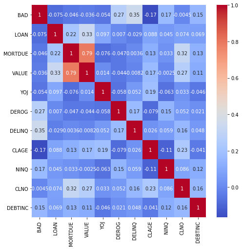
We can check correlation with the target variable using a simple Heatmap.

f, ax = plt.subplots(figsize=(8, 8))
ax = sns.heatmap(df.corr(),
            cmap = 'coolwarm', 
            annot = True)

WOE transformation

Next we will transform our variables into WOEs. To do that, we will use 2 python libraries: scorecardpy and Monotonic WOE Binning. The reason to use both packages is that, while the former will perform the whole sequence of transformation-estimation-performance analysis, the latter will assure the monotonicity property of WOEs.

Let’s go ahead and import the libraries

#!pip install scorecardpy
#!pip install monotonic-binning
import scorecardpy as sc
from monotonic_binning.monotonic_woe_binning import Binning

Data Split and WOE computation of numeric variables

We will define a function to compute numeric variables with the monotonic_binning package.

# Perform a 70 / 30 split of data
train, test = sc.split_df(df, 'BAD', ratio = 0.7, seed = 999).values()

# Function to compute WOEs
var = train.drop(['BAD', 'REASON', 'JOB'], axis = 1).columns
y_var = train['BAD']

def woe_num(x, y):
  bin_object = Binning(y, n_threshold = 50, y_threshold = 10, p_threshold = 0.35, sign=False)
  global breaks 
  breaks = {}
  for i in x:
    bin_object.fit(train[[y, i]])
    breaks[i] = (bin_object.bins[1:-1].tolist())
  return breaks
  
woe_num(var, 'BAD')

This will return a dictionary that we will pass as argument to the scorecard package. But before that, we need to compute the WOEs for cathegorical variables.

# Check categorical variables names
bins = sc.woebin(train, y = 'BAD', x = ['JOB', 'REASON'], save_breaks_list = 'cat_breaks')
# import dictionary
from cat_breaks_20200724_164925 import breaks_list
breaks_list

# merge
breaks.update(breaks_list)
print(breaks)

WOE transformation

Finally it’s time to use the dictionary of WOE-rules and apply them to the original variables in train/test.

bins_adj = sc.woebin(df, 'BAD', breaks_list= breaks, positive = 'bad|0') # change positive to adjust WOE to ln(GOOD / BAD)
# converting train and test into woe values
train_woe = sc.woebin_ply(train, bins_adj)
test_woe = sc.woebin_ply(test, bins_adj)

# Merge by index
train_final = train.merge(train_woe, how = 'left', left_index=True, right_index=True)
test_final = test.merge(test_woe, how = 'left', left_index=True, right_index=True)

And now we are all set to estimate a model! Before that, some useful tips:

• Notice that we are computing WOE = ln(good/bad), by changing the positive parameter of the woebin function.
• Take into account that we need to fill the missing values if we decide to keep the original variables (as well as the transformed ones).
  
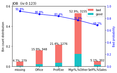
• You can manually adjust the cut-offs by calling the woebin_adj method, and you can visually inspect the new variables with woebin_plot. An example of this plot is presented below.

Logistic Regression

1. Data split and model fit

Let’s fit a Logistic Regression for the database we constructed.

# Data split
y_train = train_final.loc[:,'vd']
X_train = train_final.loc[:,train_final.columns != 'vd']
y_test = test_final.loc[:,'vd']
X_test = test_final.loc[:,train_final.columns != 'vd']

# LR fit
# logistic regression ------
from sklearn.linear_model import LogisticRegression
lr = LogisticRegression(penalty = 'l1', C= 0.9)
lr.fit(X_train, y_train)
print(lr.coef_)

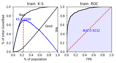
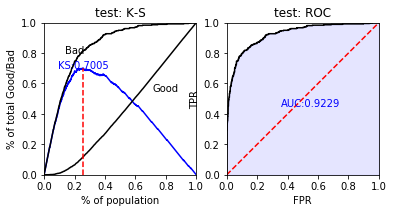
2. Performance

The scorecard package has some in-built methods to analyze performance

# predicted proability
train_pred = lr.predict_proba(X_train)[:,1]
test_pred = lr.predict_proba(X_test)[:,1]

# performance ks & roc ------
train_perf = sc.perf_eva(y_train, train_pred, title = "train")
test_perf = sc.perf_eva(y_test, test_pred, title = "test")

Performance Scores Train / Test

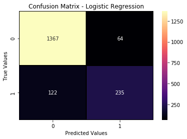
print(classification_report(y_test,predictions))

Finally we can check Precision, Recall and the Confusion Matrix

              precision    recall  f1-score   support

           0       0.92      0.96      0.94      1431
           1       0.79      0.66      0.72       357

    accuracy                           0.90      1788
   macro avg       0.85      0.81      0.83      1788
weighted avg       0.89      0.90      0.89      1788

conf_log2 = confusion_matrix(y_test,predictions)
sns.heatmap(data=conf_log2, annot=True, linewidth=0.7, linecolor='k', fmt='.0f', cmap='magma')
plt.xlabel('Predicted Values')
plt.ylabel('True Values')
plt.title('Confusion Matrix - Logistic Regression');

Wrap up

This entry presented an easy way to calculate WOEs and fit a simple model for Finance and Credit analysis. I’m aware that there are many things missing from the analysis (variables selection by IV, hyperparameters tuning, among others) but I wanted to focus only on the key steps to increase performance by transforming variables to WOEs. If you have a better way to deal with these issues, or you’ve been implementing a better solution, please contact me so that I can learn from your progress.

Extras

• Jupyter notebook of the project.
• An open repo that deals with WOE transformation through a series of functions.